Gradient descent is quite possibly the most well-known machine learning algorithm. Similarly, linear regression is present in most areas of machine learning (such as neural nets). Hence, whether you want to predict outcomes for samples, find a local minimum to a function or learn about neural networks, you will certainly come across gradient descent.
This post aims to make the maths and implementation of gradient descent as clear as water, so hopefully, you will understand the intuition behind this algorithm.
Gradient Descent Overview
Luckily for you, I’ve split this post into different sections so you don’t have to waste time on the boring stuff if you don’t want to.
Interestingly, I put all the maths involved in deriving the gradient descent algorithm in a video. Hopefully, this makes things a little easier to either understand or skip past. In addition, the Python code is all on Github, in case you just want to go straight to the code.
The contents list below summarises the sections of this post.
- Intuition behind gradient descent
- Deriving gradient descent for linear regression
- Implementing gradient descent in Python, Pandas and Numpy
- Get the code on Github.
How Does Gradient Descent Work? The Intuition Behind It
As you may know, linear regression is about fitting a line through a set of points. More specifically, the fitted line must be very good at predicting. Therefore, we want the difference between our predictions and the actual values (outputs) of the dataset to be as low as possible.
Defining The Cost Function For Linear Predictions
Gradient descent begins with the definition of a cost function. But what is this cost function? Well, for linear regression, we define the cost function as the sum of the squared errors of our predictions. In other words, the cost function is the difference between the predicted values a line will give us, and the actual output in the dataset, squaring the result at the end.
\textbf{C}(\mathbf{\utilde{w}}) = \sum_{i=1}^m {(y_i-\mathbf{\utilde{w}}^T\mathbf{\utilde{x^i}})^2}Let’s dive into what the cost function above means. Firstly, we’re assuming that we have m samples. Each sample \mathbf{\utilde{x^i}} = [1\ x^i_1\ x^i_2\ ...\ x^i_n]^T has a one in the first dimension, and n other components following that. Similarly, \mathbf{\utilde{w}} = [w_0\ w_1\ w_2\ ...\ w_n]^T is the vector of weights for the line.
In addition, both \mathbf{\utilde{w}} and \mathbf{\utilde{x}^i} are (n+1,1) vectors. The former is a representation of our line (w_0 is the constant term, and the later is a particular sample in our dataset, x^i_0 is always 1 to account for the constant term).
So basically, \mathbf{C}(\mathbf{\utilde{w}}) tells us “how good” our line is at predicting samples we already know the result for.
Ok, so how does a cost function help us find the perfect \mathbf{\utilde{w}} for our prediction line?
Gradient Vectors Guide Us To The Right Direction – Linear Regression Made Easy
If you’re familiar with calculus and linear algebra, you probably know about gradient vectors. Sometimes denoted with \nabla, it simply tells you the direction a curve is going to in an n-dimensional space.
With gradient vectors in mind, the idea of gradient descent in the context of linear, is to “walk” against the increases in the cost that would be done with the current choice of \mathbf{\utilde{w}}. Since the cost function considered in this post is essentially a squared function of \mathbf{\utilde{w}}, we would always decrease the cost if we updated our future \mathbf{\utilde{w}} with a negative fraction of the current one.
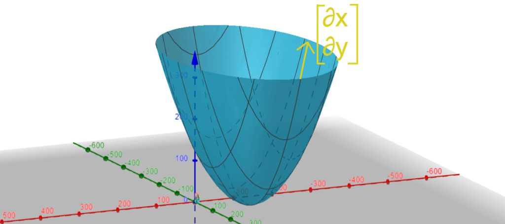
In the picture above, we have an imaginary cost function plotted in three dimensions. The yellow vector is the gradient vector at a particular point, telling us which direction the curve is going at that particular point.
Unsurprisingly, the idea of gradient descent is to find the \mathbf{\utilde{w}} with the lowest cost function, i.e. the lowest point on the curve above. Therefore, by moving opposite to the gradient vector, we can make “little steps” towards our goal.
Deriving Gradient Descent For Linear Regression – Video
The video below dives into the theory of gradient descent for linear regression. If you want to understand how the implementation actually works, I recommend watching and understanding the video lesson.
Coding Gradient Descent In Python
For the Python implementation, we will be using an open-source dataset, as well as Numpy and Pandas for the linear algebra and data handling. Moreover, the implementation itself is quite compact, as the gradient vector formula is very easy to implement once you have the inputs in the correct order.
Linear Regression Dataset – Fish Market From Kaggle
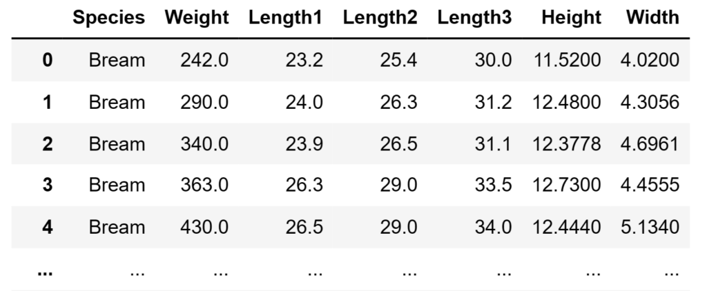
For this tutorial, you will need to download the “Fish Market” dataset from Kaggle. Briefly speaking, this dataset contains information on different fish species, and it comes as a csv file.
As far as this post is concerned, we will only consider one of the fish species in the dataset, and within this, we will only look at the “width” and “height” features as they should be fairly linearly correlated.
Installing The Dependencies – Notebook, Numpy, Pandas, And Matplotlib For Python
Most of the code in this post was written in a Jupyter Notebook, with the aid of other third-party libraries. The list below contains everything you need to install in your Python environment.
- Numpy for linear algebra.
- Pandas for viewing the data in the
csvfile. - Matplotlib for drawing the line and graphs.
- Jupyter Notebook for visualising the implementation.
I recommend using Miniconda for managing your Python environments.
Theory Used In the Implementation Of Gradient Descent For Linear Regression
Without further ado, the star of the show this post is the equation for calculating the gradient vector of the current cost function with respect to the line weights. The block below shows the equation.
\begin{align}
\nabla\mathbf{C(\utilde{w})}\quad &=\quad

\begin{bmatrix}
\frac{\partial\mathbf{C}}{\partial\mathbf{w_0}} \\
\frac{\partial\mathbf{C}}{\partial\mathbf{w_1}} \\
\vdots \\
\frac{\partial\mathbf{C}}{\partial\mathbf{w_n}}
\end{bmatrix}
\\
&= \quad
-2\mathbf{X}^T(\mathbf{\utilde{y}} - \mathbf{X}\mathbf{\utilde{w}})
\end{align}
For more information on the equation above, watch the video about deriving the maths behind gradient descent.
Specifically, the equation above assumes that you have the dataset in the correct format. For instance, you need to construct the following matrices and vectors.
\mathbf{X} =
\begin{bmatrix}
  \sim \mathbf{\utilde{x}^1} \sim \\
   \sim \mathbf{\utilde{x}^2} \sim \\
  \vdots \\
   \sim \mathbf{\utilde{x}^m} \sim \\
\end{bmatrix}
=
\begin{bmatrix}
  1 & x^1_1 & x^1_2 & ... & x^1_n \\
  1 & x^2_1 & x^2_2 & ... & x^2_n \\
  \vdots & \vdots & \vdots & \ddots & \vdots & \\
  1 & x^m_1 & x^m_2 & ... & x^m_n
\end{bmatrix} \\

\mathbf{\utilde{y}} =
\begin{bmatrix}
  y_1 \\ y_2 \\ \vdots \\ y_m
\end{bmatrix},

\mathbf{\utilde{w}} =
\begin{bmatrix}
  w_0 \\ w_1 \\ \vdots \\ w_n
\end{bmatrix},

\mathbf{\utilde{x}}^i =
\begin{bmatrix}
  x^i_0 \\ x^i_1 \\ \vdots \\ x^i_n
\end{bmatrix} =
\begin{bmatrix}
 1 \\ x^i_1 \\ \vdots \\ x^i_n
\end{bmatrix}
Briefly speaking, \mathbf{X} is an (m, n+1) matrix where each row is a sample in your dataset (without the outcome).
The outcomes vector, \mathbf{\utilde{y}}, is an (m,1) vector with the outcomes in the dataset, that matches each of the rows in \mathbf{X}.
Finally, \mathbf{\utilde{w}} and \mathbf{\utilde{x}^i} are both (n+1,1) vectors. The former is the weights of our line, and the latter is the i^{th} sample in our dataset, with an added constant one as the first component.
Loading And Visualising The Dataset With Jupyter Notebook And Python
Initially, we load the dataset. Assuming you downloaded the “fish_market.csv” from Kaggle, place it somewhere in your computer and use the following code to load and display the dataset on Jupyter Notebook.
%matplotlib inline
import cv2
import numpy as np
import pandas
from matplotlib import pyplot as plt

# from https://www.kaggle.com/aungpyaeap/fish-market
fish_csv = pandas.read_csv("C:PATH\\TO\\fish.csv")
fish_stats = fish_csv[fish_csv["Species"] == "Bream"]
fish_stats = fish_stats[["Width", "Height"]].to_numpy()

plt.scatter(fish_stats[:,0], fish_stats[:, 1])
fish_csv
As you can probably tell, the code above loads the csv dataset with Pandas, then selects the “Width” and “Height” samples for all the “Bream” species entries. We then immediately turn the Pandas dataframe into a Numpy array for calculation purposes in the future.
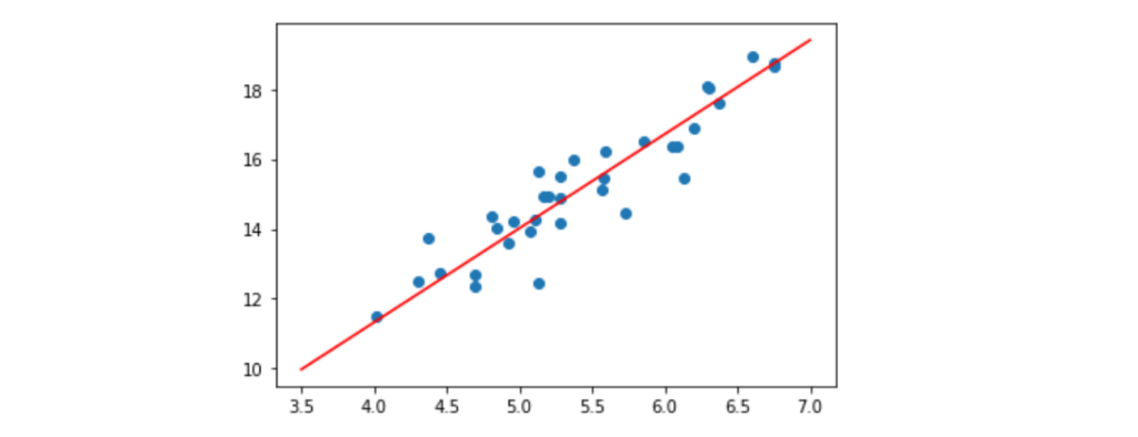
Unsurprisingly, the second to last line will plot a graph of the samples’ width and height. Following that, the last line simply asks Jupyter Notebook to display the fish_csv dataframe so we can see what the whole dataset looks like.
As you can see, the width (on x-axis) seems to be somewhat linearly-correlated to the height (y-axis). Obviously, this should be the case as the bigger width a fish has, the bigger the height is likely to be. Therefore, for this hypothetical example, we will try to predict a fish’s height based on the width.
Constructing The Matrices And Vectors Needed
Assuming you have executed the lines in the previous code block, fish_stats contains a Numpy matrix with a sample per row. Therefore, it has m rows, each row with 2 columns (width, and height, in order).
Our job is to split the fish_stats dataset into a matrix of samples (containing the widths), \mathbf{X}, and the outcomes vector \mathbf{\utilde{y}} (containing a height for each width).
Normally, \mathbf{X} would have samples with many dimensions. However, since we’re only using the width of a fish to predict the height, \mathbf{X} is essentially a column vector, where each row is the width of a fish. However, as long as the input matrix to the code in this section has a sample per row in \mathbf{X}, all the code mentioned here should work.
The code below transforms a sample matrix into the final \mathbf{X} matrix with the additional ones at the start of each row.
def get_full_sample_matrix(samples):
    samples_matrix = samples.copy()
    if samples.ndim == 1:
        samples_matrix = samples_matrix.reshape(-1, 1)

    ones_vec = np.ones((samples_matrix.shape[0], 1), dtype=samples.dtype)
    return np.hstack([ones_vec, samples_matrix])
The logic is pretty simple, but the function above copies the input samples to samples_matrix, turns it into a two-dimensional vector if it’s an Numpy array (with that if check), then stacks ones to the start of each row.
With the function above, we can simply use fish_stats to get our \mathbf{X} matrix.
X = get_full_sample_matrix(fish_stats[:, 0])Finally, we can get the outcome vector \mathbf{\utilde{y}} with the following line.
Ys = fish_stats[:, 1].reshape((Xs.shape[0], 1))Essentially, the line above gets the vector containing all the heights for each row of X .
Implementation Of A Gradient Descent Function
Before we start, I just want to remind you that our goal is to find the gradient vector, \nabla\mathbf{C(\utilde{w})}= -2\mathbf{X}^T(\mathbf{\utilde{y}} - \mathbf{X}\mathbf{\utilde{w}}), then “walk” towards the negative direction in the cost function. In other words, we remove a fraction of the gradient from the current \mathbf{\utilde{w}}.
def grad_desc(Xs, Ys, rate = 0.001, iterations = 100):
    w = np.zeros((Xs.shape[1], 1))
    for _ in range(iterations):
        errors = Ys - Xs.dot(w)
        grad = -(Xs.T).dot(errors)
        w = w - rate*grad
    return w
Believe me or not, the code above is everything we need to implement gradient descent. The inputs are explained in the list below.
Xsis the input samples matrix, with the added ones at the start of each row.Ysis the outcome vector. Each row should be the outcome for the equivalent row inXs.rateis the fraction of the gradient to subtract from \mathbf{\utilde{w}}, on each iteration. Defaults to 0.001.iterationsis the number of times we will calculate the gradient vector, and subtract it from the current \mathbf{\utilde{w}}. Defaults to 100.
There’s not much to say about the function grad_desc(...), it simply implements the theory we’ve looked at. However, you may have noticed that, we essentially only find -\mathbf{X}^T(\mathbf{\utilde{y}} - \mathbf{X}\mathbf{\utilde{w}}), in other words, half of what \nabla\mathbf{C(\utilde{w})} should be. Due to being able to set the learning rate, I decided to remove that extra multiplication as we can simply reduce the value of rate instead.
Lastly, let’s just look at the initial value of w in that function. On line 2, w starts with zero values for every component. You may be wondering why, but essentially, the initial value of w doesn’t matter, as we update each component to be a step closer to best value with each iteration of the gradient descent.
Using The Gradient Descent Function To Find Out Best Linear Regression Predictor
We have the function for “machine learning” the best line with gradient descent. Using it with the dataset and matrices we’ve constructed is very easy.
w = grad_desc(Xs, Ys)The line above will find the best possible vector \mathbf{\utilde{w}} to represent our prediction line.
Interestingly, it uses the default value for rate (0.001) and iterations (100). These values do work well for the dataset considered in this post, however, for different datasets, you may want to experiment with different learning rates and iterations.
There are many posts on the internet regarding which values are best to pick, so I’ll let you do your own research on the trade-offs between big vs small learning rates/iterations.
Plotting The Prediction Line Against The Original Samples
Now that we can learn the best line, lets use it to plot the prediction line against the original samples.
line_ends = np.array([3.5, 7.0]).reshape(-1, 1)
prediction_Xs = get_full_sample_matrix(line_ends)
prediction_Ys = (prediction_Xs).dot(w)

plt.plot(line_ends, prediction_Ys, color="red")
plt.scatter(fish_stats[:,0], fish_stats[:, 1])
Unsurprisingly, when you add the code above to Jupyter Notebook, you should see a scatter (in blue) of the original samples, as well as a red line representing our prediction.
Most importantly, the previous code block shows how to do predictions. In order to get the endpoints for the line, I created a sample matrix line_ends with the first and last “samples” I’d like to predict. Lines 2 and 3 show how to go from a matrix of samples (in each row) to a vector of predictions.
As an exercise to the reader, you can create a function that takes samples and gives out a vector of predictions. Feel free to post your solution in the comments, I’ll tag the first correct-looking solution in this post!
Getting The Code On Github
The entire Jupyter Notebook containing all the code mentioned in this post can be found here.
Just bear in mind that you will need to install all the dependencies we previously mentioned. If you find any issues with the code, feel free to either comment down below or raise an issue on Github.
Check Out Other Related Python Articles!
This article is part of a series of Python implementation posts, where we talk about the theory of something, and then implement it! If you’re interested, check out the last post of the series on how to implement Conway’s game of life.
If you prefer more mathematical articles, check out my post on implementing the trapezium rule in Python.
Did I miss anything? Did you spot any mistakes in the post? Do you have feedback? Feel free to comment below and I’ll get back to you as soon as possible!
Be First to Comment