The trapezium rule is part of most maths-related course syllabuses out there. Whether you’re studying engineering, computer science, or pure maths, you will come across the trapezium (or trapezoidal) rule. In this post, we will learn how to use Python to implement and automate the trapezium rule!
Trapezium Rule – A Recap
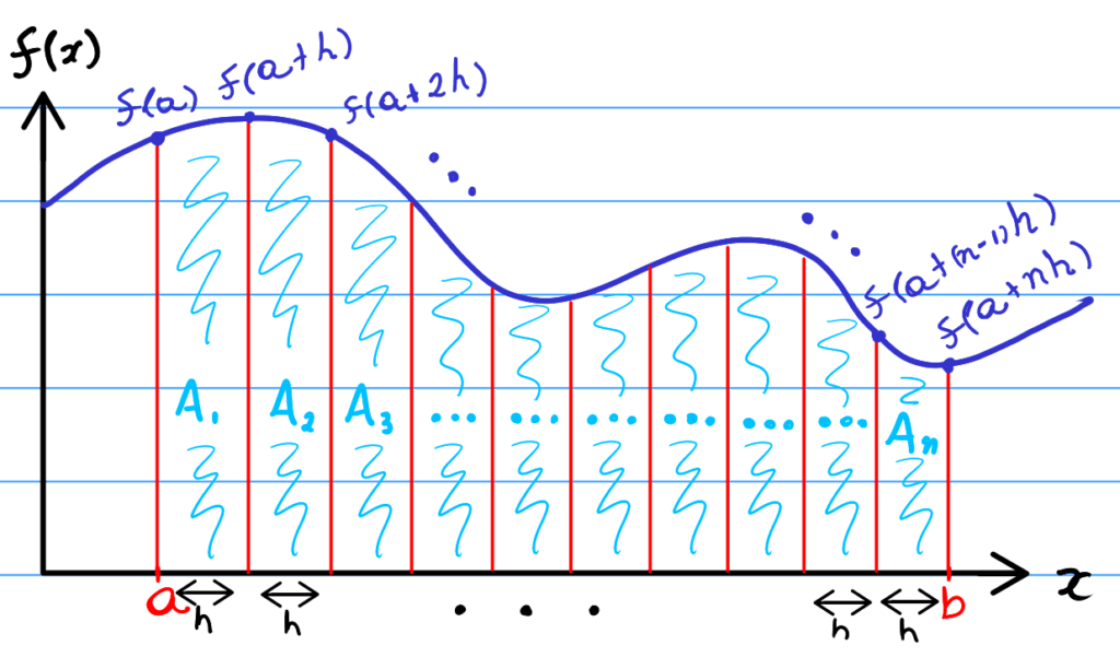
The trapezium rule is very useful if you need to estimate the area under a curve for a set of inputs and samples for a function.
Interestingly, you do not necessarily need to know the formula of the function. However, you must know the outputs of the function sampled at regular intervals (height of the trapezium).
If you are not familiar with or do not completely understand the trapezium rule, read my previous post on how to understand the trapezium rule. It won’t take long and it will help you understand the logic behind this rule!
What Do I Need To Implement The Trapezium Rule?
In this post, we will be using Python to implement the trapezium rule. In addition, will implement it in a few different ways and compare how efficient each implementation is.
For the purposes of this post, I recommend installing Miniconda with the latest version of Python available if you do not already have it. Miniconda is a Python environment manager that allows you to easily have different Python installations and different libraries.
Setting Up The Enviroment And Tools
Once you have installed Miniconda in your system, you need to open the “Anaconda Prompt” command line and create an environment for our experiment in this post. Simply type in the following commands in the “Anaconda Prompt”:
conda create --name maths python=3.9
conda activate maths
conda install numpy
To quickly explain the commands above:
- Line 1 creates a new Python environment called “maths” with Python 3.9. Obviously, if there are newer versions of Python by the time you’re reading this, feel free to change the version.
conda activate mathsloads up the environment we just created. When activated, any tools or libraries we install will be added to the “maths” environment.conda install ...will get and install the specified libraries/tools to the activated environment. In our case, we need thenumpylibrary for mathematics.
Hopefully, all the commands worked just fine and you’re all set! Otherwise, drop a comment with the errors you have and I’ll try to help you.
A Pure Python Implementation
In this section, we will implement the Trapezium Rule solely with Python and its standard library. Although this will be the least efficient implementation, at least compared to the Numpy counterparts, it gives a better insight into how these types of algorithms are implemented. So I would recommend typing out this solution and understanding the techniques used here!
Creating The Input Samples Array
To begin with, we need to create an array of outputs to the function we want to estimate the area for with the Trapezium Rule. For a quick recap, if we want to estimate the area with N trapeziums in the interval [a,b], then we need N+1 equally spaced outputs.
So let’s begin with creating the sample inputs (the x values).
def get_input_samples(first_x, last_x, N):

    # Height of the trapeziums, or dx
    h = (last_x - first_x) / N
    return [first_x + i*h for i in range(N+1)]
Given the first and last inputs, a and b, the function above will return a list of N+1 samples equally spaced by the height of each triangle, h or dx. Furthermore, the first element will be a and the last will be b. You can work it out mathematically if you want.
Creating The Output Samples
Once the equally spaced inputs are calculated, getting the output array is easy, as shown in the code below.
def apply(f, inputs):
     """
     This will apply the function f on each
     elements of inputs.
     """
     return [f(x) for x in inputs]
Interestingly, the function above is called apply because it applies the function f(...) to each element in the inputs list.
Admittedly, this code can be quite strange to beginners because we are passing a function as an input to another function, but that is quite a good feature of Python. So when we say we “apply” the function to each input, it simply means that we call that input function with each element of the inputslist as a parameter.
For example, say we have the list of inputs [1, 2, 3, 4, 5, 6], then if we call apply(lambda x: x**2, [1, 2, 3, 4, 5]) would return [1, 4, 9, 16, 25, 36].
Getting The Final Result
Putting two and two together, we can now use the functions we implemented to get the trapezium rule result for an array of samples.
To recap from the post about explaining the trapezium rule, given a set of equally spaced samples for a function, the trapezium rule tells us the following:
\int_{a}^{b} f(x) dx \approx \frac{h}{2} \{f(a) + f(b) + 2[f(a+h) +\cdots+f(a+(n-1)h)]\}The following function does just that: it takes an array of samples and the height of the trapezium (the width of each sample), and returns the integration estimate using the trapezium rule.
def trapezium_rule(samples, h):
     """
     Apply the trapezium rule to the samples
     array with the samples equally spaced
     with the value of h.
     """
     return (h/2) * (samples[0] + samples[-1] + 2 * sum(samples[1:-1]))
If you simply want to estimate the derivative of a function between two points, we can define a function to do that with the trapezium rule:
def estimate_area(f, first_x, last_x, N):
     """
     Gets the estimate for the area of "f" using
     the trapezium rule with "N" trapeziums starting
     in the interval ["first", "last"].
     """
     inputs = get_input_samples(first_x, last_x, N)
     samples = apply(f, inputs)
     dx = (last_x - first_x)/N
     return trapezium_rule(samples, dx)
So given a function-like object f (such as lambdas), the first and last sample points (a and b), and the number of trapeziums N, estimate_area(f, a, b, N) will return the estimate using the trapezium rule. Voilà!
For example, estimate_area(lambda x: math.e**(-x**2), -10, 10, 100) returns the amazing estimate of 1.7724538509055154. Hopefully, you can see how good this estimate is if you know anything about the integral of \int_{-\infty}^{\infty} e^{-x^{2}} dx.
A Naive Numpy Implementation
Any scholar or data scientist will question the “pure” Python implementation, and wonder why we’re not using Numpy, a library built for heavy-weight mathematics.
Cutting to the chase, we can use Numpy arrays and functions to create a faster implementation of the estimate_area(f, a, b, N) function:
# Needed to use numpy functions and arrays
import numpy as np

def estimate_area_numpy(f, a, b, N):
     """
     Returns the area estimate using the
     trapezium rule, using numpy arrays
     and functions.
     """
     # Calculate the trapezium height
     h = (b-a)/N
     # Get the array of inpus (x-values)
     Xs = np.linspace(a, b, N+1)
     # Evalueate the function on inputs
     Ys = f(Xs)
     return (h/2) * (Ys[0] + Ys[-1] + 2*np.sum(Ys[1:-1]))
Interestingly, the function above does the same as estimate_area(f, a, b, N), but it uses Numpy to create the input and output arrays. Note that the input function f needs to handle a whole Numpy array input! So stick to the Numpy functions.
Finally, to calculate the same integral as the “pure” Python implementation would be estimate_area_numpy(lambda Xs: np.exp(-Xs*Xs), -10, 10, 100) . Note how the input function uses np.exp(...), which handles the entire Numpy array at once, making it more efficient. Needless to say, it returns the same estimate.
An Even Smaller Trapezium Rule Numpy Implementation
Would you believe we can do all of the above implementations in just three lines of code? Due to Numpy providing us the trapz(Ys, Xs, ...) function, we could directly rely on Numpy to apply the trapezium rule on a set of samples! The code below shows how.
def estimate_area_numpy_trapz(f, a, b, N):
     Xs = np.linspace(a, b, N+1)
     Ys = f(Xs)
     return np.trapz(Ys, Xs)
np.trapz(Ys, Xs) will use Numpy’s own implementation of the trapezium rule. However, because it is implemented in native code, with highly optimised routines, it will smoke the other approaches shown in this post in terms of efficiency!
Obviously, estimate_area_numpy_trapz(lambda Xs: np.exp(-Xs*Xs), -10, 10, 100) will return the same estimate as the others.
Benchmarking Different Implementations Of The Trapezium Rule
As I was curious about knowing how much better the Numpy implementations were from the “pure” Python ones, I decided to benchmark all the trapezium rule functions we created in this post. In addition, they are all estimating the integral for the same function, namely f(x) = e^{-x^{2}}. However, I’ve changed the first and last input points (the integral bounds a, b), and the number of trapeziums N.
| Input {a, b, N} | estimate_area Pure Python | estimate_area_numpyNaive Numpy | estimate_area_numpy_trapzNumpy all the way |
|---|---|---|---|
{-10, 10, 100} | 50.4 µs | 38.6 µs | 48.8 µs |
{-10, 10, 1000} | 507 µs | 46 µs | 58.7 µs |
{-15, 15, 10000} | 4.89 ms | 113 µs | 140 µs |
{-15, 15, 20000} | 9.93 ms | 188 µs | 229 µs |
{-20, 20, 50000} | 26.1 ms | 928 µs | 1.03 ms |
np.traz(...). Unsurprisingly, the “pure” Python implementation is very slow compared to the Numpy counterparts. In cases where the number of trapeziums is big, we see a 20x slowdown.
So there nothing unexpected in that sense. However, I wrongly assumed that the np.trapz(...) function would be faster than our naive Numpy extimator. As we can see, both functions nearly go toe-to-toe on efficiency, but np.trapz(...) does lose to the naive Numpy counterpart by a little bit in every scenario. I’ve even double triple checked it!
Goes to show you: benchmark your code before making any assumptions!
TL;DR
We have seen in this article how easy it is to implement the Trapezium Rule purely in Python.
Furthermore, this task becomes even easier (and more efficient) when using a numerical library such as Numpy.
Benchmarks show us that, in the worst case scenario, the “pure” Python implementation performed twenty times worse than the Numpy implementations. In addition, they also show us that a naive Numpy, which performs the Trapezium Rule with Numpy arrays and functions in Python lines, did actually perform better than Numpy’s own np.trapz(...) function (by a little).
Do I think the “pure” Python implementation is useless? No, quite the contrary. Knowing how to use Python to implement mathematical methods is useful; it gives you an insight into what people have to do when writing the same thing in other languages. It wouldn’t surprise me if Numpy actually implements the same formula in native code (C/C++), with some optimisations.
In fact, it’s certainly useful to know how something is implemented. It helps you understand a concept better!
Did I miss anything? Spotted any mistakes in the writing or code? Do you have any questions? Please post a comment below and I’ll try my best to reply ASAP!
Be First to Comment