Have you ever had to estimate the integral of a complex curve/function? The trapezium rule is a very easy numeric method to understand and apply. In this post, I will be going over how to derive the rule and how to use it in an easy manner.
Integration: The End Goal
Before getting into the nitty-gritty of numerical integration, we need to understand the main goal of integration: finding the area under a curve with a known equation.
But how do we calculate the exact area of such a curve? For the purposes of numerical integration, we do not care! In this post, we’re only concerned with finding the area of a function, given that you have a set of inputs and outputs to it. We don’t even need to know the equation for the function!
Of course, if you have taken any calculus courses at school, you should already be familiar with a few methods and identities you can use to integrate equations. But we will not discuss those methods here.
To summarise, you should have only one thing in mind: finding the area under a curve given a set of inputs and outputs.
Understanding The Trapezium Rule
The trapezium rule is actually very easy to understand once we understand the problem. So let’s begin talking about (and visualising) integration.
The Need For Numerical Integration
As we know, integration is about finding the area between a curve (or function) and the x-axis. Figure 1 shows the area we need to calculate for a random function f(x) .

As we know from calculus, there are functions for which you can find the exact value of the area between limits [a,b]. This works well if it’s a basic function and if you know the antiderivatives. But what about more complicated functions? What if a function doesn’t have an antiderivative? Something like g(x) = e^{x^2}? What would \int_{a=0}^{b=10} g(x) dx be?
This is where the trapezium rule, or more generally numerical integration, becomes handy. When the function/curve has a complicated formula but you can calculate outputs from inputs, then you can apply numerical integration.
Just bear in mind that numerical methods will not give you the exact area, but a good enough estimate. And you will see why.
Deriving The Trapezium Rule
Assuming that you are able to calculate output values for a function, say f(x), and that for any x \in [a,b], f(x) exists (i.e. if f(x) is well-defined for any input in the interval [a,b]), we can use the trapezium rule.
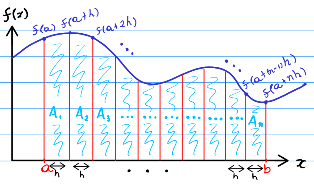
Explaining the idea is very simple. For any given function f(x), and the interval [a,b] where we would like to estimate the area of f(x), we can instead split the area into separate, non-overlapping areas. This is represented by A_1, A_2, \cdots, A_n.
In addition, each area A_i has the width h. Luckily, h can be easily calculated depending on how many area sections you want. For example, if we want to divide the area of f(x) between [a,b] into 4 equal-width sections, we can use h= \frac{b-a}{4}. More generally, h = \frac{b-a}{n}, where n is the number of sections we want.
Finally, the idea of the trapezium rule is to estimate each section A_i as the trapezium made by the x-axis and the corner values of f(x). For example, A_2 would be estimated as the area of the trapezium enclosed by the points (a+h, 0), (a + 2h, 0), (a + 2h, f(a + 2h)), and (a +h, f(a + h)). The figure below demonstrates this idea.
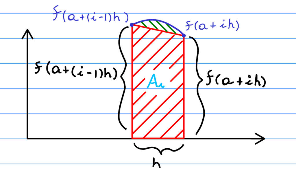
As you probably guessed, the general estimated area of A_i is calculated from the trapezium formed by (a+(i-1)h, 0), (a + ih , 0), (a + ih, f(a + ih)), and (a + (i-1)h, f(a + (i-1)h)). We’re using i as an integer here, not the imaginary number!
The Equation For The Trapezium Rule
From the above assumptions and explanations, you can now fully understand the formula. But before we look at the trapezium rule, let’s be clear of somethings.
In our examples, we’re assuming that we have n trapeziums. These trapeziums have a height h. This height is constant and dependent on the integration interval and the number of trapeziums. Finally, the bases of the trapezium are given by the values of f(x) evaluated at both “ends” of our trapeziums. For example, f(x + h) and f(x + 2h) for A_2.
The formula for the area of a trapezium is
\begin{aligned}
    A = \frac{b_1 + b_2}{2}h
\end{aligned}
where the bases \{b_1, b_2\} are \{f(x+(i-1)\delta x),f(x + i\delta x)\} and the height (h) is the same height shown in the examples. for this reason, the whole area for f(x), between interval [a,b] and n trapieziums is
\begin{aligned}
    \int_a^b f(x) dx
    \approx \sum_{i=1}^n A_i
    = \sum_{i=1}^n  \frac{f(a+(i-1)h) + f(a+ih)}{2}  h
\end{aligned}
Here, we change the meaning A_i slightly to the area of the i^{th} trapezium created from our function split.
Interestingly, if we rearrange the sum above and expand it, we have the following
\begin{aligned}
    \int_a^b f(x) dx
    &\approx \frac{h}{2} \sum_{i=1}^n f(a + (i-1)h) + f(a + ih)\\
    &\approx  \frac{h}{2} [(f(a) + f(a+h) ) + (f(a+h) + f(a + 2h)) + \cdots \\
    &\qquad + (f(a + (n-2)h) \\
    &\qquad+ f(a + (n-1)h)) + (f(a + (n-1)h) + f(a + nh))]
\end{aligned}
Finally, the pattern is that most of the terms inside the above sum show up twice, with the exception of f(a), and f(a+nh) = f(b) (as a+nh = b). Therefore the trapezium rule becomes:
\begin{aligned}
\int_a^b f(x) dx &\approx \frac{h}{2}\{f(a) + f(b) + 2[f(a + h) + \cdots + f(a + (n-1)h)]\}
\end{aligned}
A Note On Error
Unfortunately, the trapezium rule doesn’t quite give you the exact area. As you can see from Figure 3, the trapezium we constructed leaves out (or adds) some area from the true area of that curve’s section. For this reason, the green proportion of Figure 3 is the error, and each trapezium in our estimation will have some error associated with it.
Interestingly, the more trapeziums we have in our estimation, the less the error value is. Consequently, increasing the value of n, in turn increasing the number of samples from f(x), will improve the estimation.
In addition, the error may not be an issue if you are using the trapezium rule on a linear function (straight-line). I’ll leave this up to you to figure out why!
Using The Trapezium Rule
If you got through the article and understood everything so far: congratulations! But you might be wondering: how do we use the trapezium rule? It’s actually very easy, we just need to match the equations we derived into data.
Let’s use an example. Firstly, we’re going to estimate the integral of e^{-x^2} between -10 and 10. Let’s say we want to estimate this with n=100 trapeziums.
Then we have the following:
\begin{aligned}
&a = -10 \\
&b = 10 \\
&n = 100 \\
h = \frac{b-a}{n} &= \frac{10 - (-10)}{100} = 0.2 \\
\end{aligned}
Now we need to calculate the values of f(a), f(a+h), \cdots, f(a + (n-1)h), f(a+nh) = f(b). This is very easy, we simply calculate the input array for x, i.e. \{a, a + h, a+2h, \cdots, a + (n-1)h, a + nh = b\}, and work out f(x) for each of these! In other words, we should have the following arrays:
\begin{aligned}
    &\{a, a+h, a+2h, \cdots, a + (n-1)h, a + nh = b\} \qquad\textbf{x inputs}\\
    &\{f(a), f(a+h),\cdots, f(a+(n-1)h), f(a+nh) = f(b)\} \quad\textbf{f(x) outputs}
\end{aligned}
In my example, where f(x)=e^{x^2}, a = -10, b=10, h = 0.2, I calculated the following:
\begin{aligned}
    &\{-10, -9.8, -9.6, \cdots, 9.8, 10\} \qquad\textbf{x inputs}\\
    &\{f(-10), f(-9.8),\cdots, f(9.8), f(10)\} \quad\textbf{f(x) outputs}
\end{aligned}
As you can see, I omitted the values of f(x) outputs above as they are quite long numbers (in terms of scientific notation). Hence, instead of showing truncated numbers and losing precision, I’m hoping that you understand what needs to be done! A good old calculator session to workout those values!
Putting It All Together With The Trapezium Method
Finally, putting it all together with the trapezium rule, we have:
\begin{aligned}
    \int_{-10}^{10} e^{-x^2} dx &\approx \frac{0.2}{2} \{f(-10) + f(10) + 2[f(-9.8) + f(-9.6) + \cdots + f(10)]\} \\
    &\approx 1.7724538509055154
\end{aligned}
In fact, this is astoundingly close to the actual value given using other calculus techniques! By the way, the integral \int_{-\infty}^{\infty} e^{-x^2} dx = \sqrt{\pi}. So this little experiment gave us an amazing estimate to that as well!
Coding The Trapezium Rule
If you’re interested in Python, look at how to implement the Trapezium Rule with Python. Similarly, if you are interested in seeing how to implement this idea in C++, check out my post on implementing the trapezium rule in C++!
I hope you understood everything in this post, if not, feel free to ask questions in the comments!
Did I miss anything? Got any feedback/questions regarding the post? Use the comment section below!